Visualizing CGAffineTransforms
Lately I have been watching the excellent “Essence of Linear Algebra” video series by 3blue1brown. As an iOS developer, I was vaguely familiar with CGAffineTransform and how it could be used to scale, rotate and shear UIViews. Watching 3b1b’s series helped me understand the math behind it. This post is my attempt at explaining, and cementing my own understanding, of the concept.
What is a transform?
A transform is, quite simply, transformation of space. Take a piece of paper lying on a flat table. This paper represents our sample space. Assign an arbitrary point on this paper as origin. We can rotate the paper about the origin, stretch it in all directions (assuming our paper is made out of rubber), move the paper around or go fancy and curl it up into a cylinder. Each of these actions represents some sort of transform we performed on our “space”.
Linear Transforms
Before looking at affine transforms, let’s look at a subset of it called linear transforms. A linear transform is a transform subject to following restrictions -
- All lines must remain lines
- Origin must not move
We will concern ourselves with two dimensional spaces in this article. A 2D space can be represented using a grid wih X and Y axes. Following are examples of transforms on this grid which are NOT linear. Blue grid lines denote the space after transform and light gray lines in background denote the original un-transformed space. White lines are X and Y axes.
Non linear transform. Lines get all curvy. Non linear transform. Origin moves. Non linear transform. Diagonal line gets curvy
Given these restrictions, how would you go about expressing a linear transform numerically? To do this, imagine two special vectors - $\hat{i}$ and $\hat{j}$ lying along postive X and Y axes respectively. In iOS, positive Y axis points downwards rather than upwards, so these vectors plotted in a 2D space look something like this -
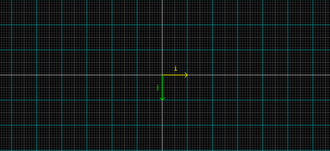
Unit vectors.
Co-ordinates of $\hat{i}$ are (1, 0) and those of $\hat{j}$ are (0, 1). When written down as row vectors -
$$ \hat{i}=\begin{bmatrix}1 & 0\end{bmatrix} $$
$$ \hat{j}=\begin{bmatrix}0 & 1\end{bmatrix} $$
Now, as long as the transform is linear, you only need to know where $\hat{i}$ and $\hat{j}$ end up after the transform to describe the linear transform numerically. Let’s consider an example -
A linear transform
The crosshairs here denote the position where our unit vectors end up after the transform. $\hat{i}$ moves from (1, 0) to (3, 1) and $\hat{j}$ moves from (0, 1) to (1, 2). So this linear transform can be represented by the matrix T -
$$ T=\begin{bmatrix}3 & 1\\1 & 2\end{bmatrix} $$
In general, any linear transform can be represented in matrix form as -
$$ T=\begin{bmatrix}a & b\\c & d\end{bmatrix} $$
where (a, b) denotes co-ords of $\hat{i}$ and (c, d) denotes the co-ords of $\hat{j}$ after the transform.
Given a vector $\begin{bmatrix}x & y\end{bmatrix}$ and transfrom T (which is a 2x2 matrix), the corresponding vector $\begin{bmatrix}\grave{x} & \grave{y}\end{bmatrix}$ can be found by multiplying the vector and transform matrix.
$$ \begin{bmatrix}\grave{x} & \grave{y}\end{bmatrix} = \begin{bmatrix}x & y\end{bmatrix} \times \begin{bmatrix}a & b\\c & d\end{bmatrix} $$
If all the matrix math stuff scares you, just remember what the matrix represents visually - The new co-ordinates of unit vectors $\hat{i}$ and $\hat{j}$ after the transform is applied. Let’s look at a few more examples visually.
Scale transform
Scaling is simple. We just need to move $\hat{i}$ and $\hat{j}$ further along their axes by whatever amount we want to scale in each direction.
Scale by 3 along X axis and by 1.5 along Y axis
Corresponding matrix -
$$ T=\begin{bmatrix}sx & 0\\0 & sy\end{bmatrix} $$
UIKit provides a convenient function CGAffineTransformMakeScale to create this matrix.
Note that you can specify negative values for sx and sy. What do you think the resulting transform will look like?
Rotation transform
Imagine moving $\hat{i}$ from (1, 0) to (0, 1) and $\hat{j}$ from (0, 1) to (-1, 0).
Rotate 90° clockwise
The effect is same as rotating the image 90° clockwise. For all other angles of rotation, it is simpler to use CGAffineTransformMakeRotation function which accepts a rotation angle and gives you back the correct transform matrix. To understand the math behind rotation angle, read up on Unit Circle
Shear transform
Shearing involves moving x co-ordinate of $\hat{j}$ for shear parallel to X axis or y co-ordinate of $\hat{i}$ for shear parallel to Y axis. Example -
Shear parallel to X axis
Corresponding matrix -
$$ T=\begin{bmatrix}1 & Sy\\Sx & 1\end{bmatrix} $$
There is no convenience function for creating a shear matrix in UIKit.
Affine Transforms
Remember the two restrictions we had imposed on a transform to qualify as linear? Namely -
- All lines must remain lines
- Origin must not move
If we remove the second restriction, the transform is said to be affine. This means all linear transforms are also affine transforms, but not all affine transforms are linear. Here’s an example -
Affine Transform. Origin moves to (-2, 1)
Affine transforms are easy enough to visualize. Afterall, Affine transform = Linear transform + Translation. But how do you represent this affine transform numerically?
If we represent the translation by a new vector $\begin{bmatrix}tx & ty\end{bmatrix}$ (remember that this vector just encodes the x and y co-ordinates of the translation), then we can represent the affine transform as -
$$ \begin{bmatrix}\grave{x} & \grave{y}\end{bmatrix} = \begin{bmatrix}x & y\end{bmatrix} \times \begin{bmatrix}a & b\\c & d\end{bmatrix} + \begin{bmatrix}tx & ty\end{bmatrix} $$
There’s one problem with this representation though. It involves two matrix operations - a matrix multiplication followed by matrix addition. Affine transforms are very common in UI code and it pays to have them represented using just a single multiplication matrix. To do this, we need to employ a bit of 3D trickery.
To higher dimension and back
We have been focusing on 2D spaces in this article. But the linear transforms mentioned here work equally well in 3D as well. In 3D, we have 3 unit vectors rather than 2 and we need 3 numbers to encode co-ordinates of each one of them, rather than 2.
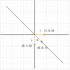
Units vectors in 3 dimensions
Let’s embed our 2D space in which the affine transform is taking place inside this 3D space. It will be a plane in this space. Let’s put this plane perpendicular to $\hat{k}$ - the unit vector along Z axis.
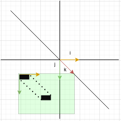
Affine in 2D is linear in 3D
Visualizing a 2D affine transform in context of this 3D space, it becomes obvious that what is an affine transform in 2D becomes a linear shear transform in 3D! And linear transforms, as we know, can be represented using a single matrix multiplication.
To help visualize this 2D affine = 3D linear trick, go back to our example of a piece of paper lying on a table. Let the floor on which the table is lying be X and Y axes and vertical be Z axis. Let the height of table be 1 unit. In this setup, the top surface of table is a plane perpendicular to $\hat{k}$. Now perform a shear operation on the whole table parallel to Z axis and observe how the piece of paper moves. It will be a translation in the 2D plane, which is the top surface of the table.
Let’s try to determine the matrix for this 3D shear transform. Our 2D linear transform equation looks like this.
$$ \begin{bmatrix}\grave{x} & \grave{y}\end{bmatrix} = \begin{bmatrix}x & y\end{bmatrix} \times \begin{bmatrix}a & b\\c & d\end{bmatrix} $$
Since we are moving up a dimension, all the matrices in this equation need to modified to account for Z axis. Let’s fill in the new values we need to introduce with ?? -
$$ \begin{bmatrix}\grave{x} & \grave{y} & ??\end{bmatrix} = \begin{bmatrix}x & y & ??\end{bmatrix} \times \begin{bmatrix}a & b & ??\\c & d & ??\\?? & ?? & ??\end{bmatrix} $$
Since we have embedded our 2D plane at (0, 0, 1) in 3D space, the value of Z co-ordinate remains constant throughout the plane. Our equation becomes -
$$ \begin{bmatrix}\grave{x} & \grave{y} & 1\end{bmatrix} = \begin{bmatrix}x & y & 1\end{bmatrix} \times \begin{bmatrix}a & b & ??\\c & d & ??\\?? & ?? & ??\end{bmatrix} $$
For the 3x3 transform matrix, rows represent co-ordinates of $\hat{i}$, $\hat{j}$ and $\hat{k}$. Z co-ordinate is zero for first two and 1 for $\hat{k}$, by definition of unit vectors -
$$ \begin{bmatrix}\grave{x} & \grave{y} & 1\end{bmatrix} = \begin{bmatrix}x & y & 1\end{bmatrix} \times \begin{bmatrix}a & b & 0\\c & d & 0\\?? & ?? & 1\end{bmatrix} $$
Last row of the transform matrix represents the co-ordinate of $\hat{k}$. Since translation in 2D is a shear in 3D - and shear parallel to Z axis will change X and Y co-ordinates of $\hat{k}$ - our equation becomes -
$$ \begin{bmatrix}\grave{x} & \grave{y} & 1\end{bmatrix} = \begin{bmatrix}x & y & 1\end{bmatrix} \times \begin{bmatrix}a & b & 0\\c & d & 0\\tx & ty & 1\end{bmatrix} $$
This equation is present in the docs of CGAffineTransform. Hopefully, this post gave you a brief idea about what the equation represents visually, and how it is derived!
Notes
- I created a small app to interactively try out various affine transforms. It can be found here
- We have been representing vectors as row matrices in this post. But that is just a convention I chose to follow since CGAffineTransform API follows the same convention. They can very well be represented as column vectors as well. In that case, we need to transpose the transform matrix and move it before the multiplication sign. i.e
$$ \begin{bmatrix}\grave{x}\\\grave{y}\\1\end{bmatrix} = \begin{bmatrix}a & c & tx\\b & d & ty\\0 & 0 & 1\end{bmatrix} \times \begin{bmatrix}x\\y\\1\end{bmatrix} $$
- You can use this website to try out linear transforms in your browser. Just keep in mind that positive Y points upwards here and matrices are transposed (see point above).